Interactive Fractal
For this demo, we want to make a fractal rendering that is navigable in real-time, with intuitive panning and zooming as if it were a large digital image. Fractal renderings that keep zooming into a predefined point are common, and offline rendering allows for fancier visual effects and much deeper zooming. However, letting the user explore it freely, in real-time, provides a different educational experience into fractals and the visual beauty of mathematics. It is also an excellent exercise in shader programming.
The Mandelbrot Fractal
One of the most famous fractals is the boundary of the Mandelbrot set, which is defined by a surprisingly simple function:
A complex number
Conveniently, the complex plane is two-dimensional, just like a computer screen. So if we plot the complex plane onto the screen, such that each pixel is given one colour if its complex coordinate belongs to the Mandelbrot set and another colour if it doesn't, we will get the simplest visualisation of the fractal curve. Doing this will already reveal the famous shape:
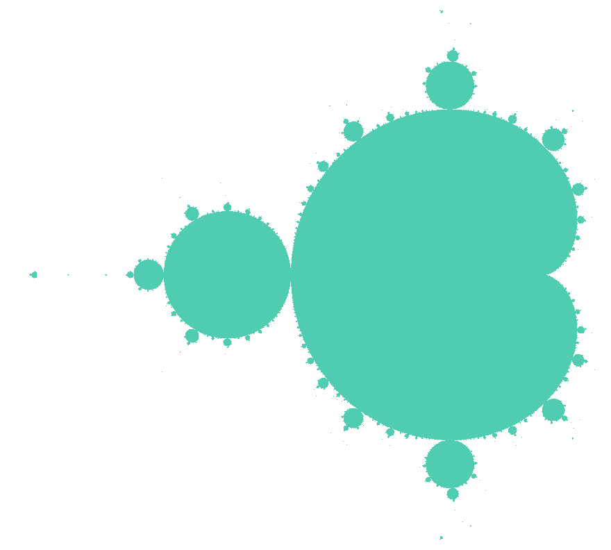
Fig. 1: The mandelbrot set in its simplest visualization: Computing whether the complex number corresponding to the coordinate of each pixel centre belongs to the set or not. Turquoise pixels belong to the set.
However, there is more to the Mandelbrot fractal than the boundary. A common visualization algorithm takes into account also the speed of divergence of each point, and visualizes it in different colours. In other words, how many times the mapping function has to be applied on a point before exiting a certain radius. Such colouring reveals some depth in the fractal:
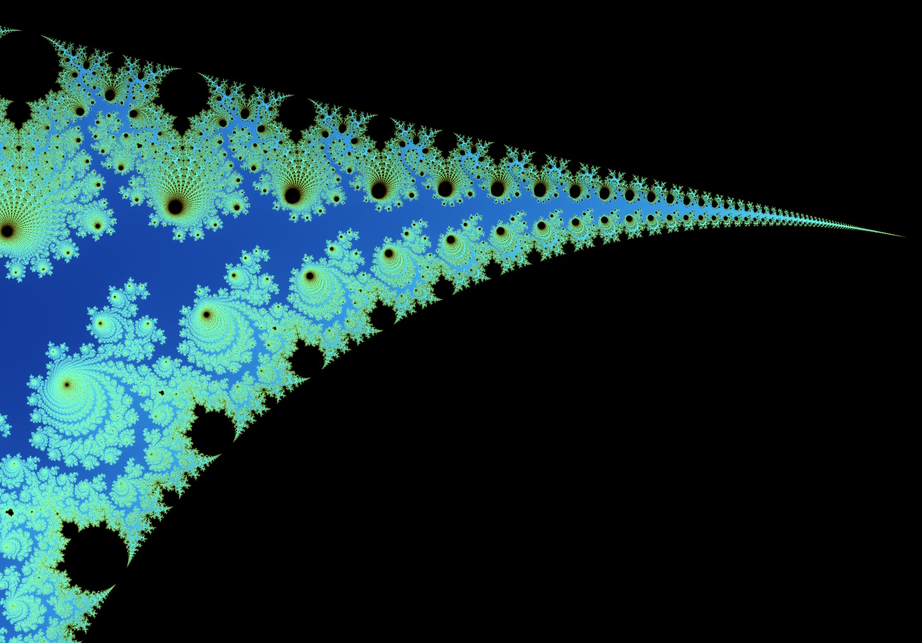
Fig. 2: Colouring based on rate of divergence. This picture is of a smaller part of the fractal, after zooming in a little.
But the real marvel of fractals is the zoom: By mapping the screen to a smaller portion of the complex plane, we achieve a zooming effect that reveals new patterns of the fractal. Mathematically, one can continue zooming indefinitely, and there are renderings that reach extreme depths and continue to reveal new and fantastic shapes and patterns. However, the deeper the zoom, the more computationally expensive it becomes to render the fractal, both because higher precision is needed in the number representations used, and because more iterations of the mapping function are needed as points diverge slower.
Implementation in WebGL
When implementing fractal visualization on a computer in practice, we obviously can't iterate our mapping functon an infinite number of times to see if it diverges. Instead, we simply pick a large enough threshold value that defines the maxumum number of iterations we will perform for each point. If after all those iterations the value still does not appear to diverge, we assume that it never will and consider it part of the set. The next step would be to define how to detect divergence. For the Mandelbrot set, it can be shown that for any point
To visualize the fractal, we need to perform this computation for each pixel. Since each pixel output does not depend on others, the computation can be done completely in parallel: A perfect problem for the GPU. In WebGL, we can simply create a screen-size quad and let the fragment shader perform the fractal computations. With a single render pass, we can both compute and visualize. In WebGL terms, it's very straight forward and requires minimal boilerplate, letting us focus our attention on the shader itself.
The GLSL code might look something like this:
vec2 squareComplex(vec2 c) {
    return vec2(c.x * c.x - c.y * c.y, 2.0 * c.x * c.y);
}

int mandelbrot(vec2 c) {
    vec2 z = vec2(0.0);
    int i = 0;
    for (; i<MAX_ITERATIONS; ++i) {
        if (dot(z, z) >= 4.0) break;
        z = squareComplex(z) + c;
    }
    return i;
}
The fractal shader calls the mandelbrot() function once, and maps the output (the number of iterations required to detect divergence) to a colour according to some colour scheme. Here, we use Bernstein polynomials to achieve a nicely weighted colour scheme in more than one hue. More complex colouring algorithms exist to e.g. prevent banding effects, but this is good enough for our purpose.
That's already most of the work. All that is left is to map each pixel to a corresponding coordinate on the complex plane. This is where navigation comes in: We want to support panning around the fractal, as well as zooming in and out in real time. The mapping function can be designed to support these navigation controls. All we actually need to uniquely identify which portion of the fractal the user is looking at is the complex coordinate at the centre of the viewport, and a radius — the distance on the complex plane from the center to the edge of the viewport. With this information, we can map linearly from pixel center coordinates to complex coordinates within the viweport. To achieve camera panning, all we need to do is move the centre coordinate, and to zoom we reduce or increase the radius. Zooming into or out from a target point (say, the cursor) can be achieved by using a combination of both.
The centre coordinate and radius are given to the fractal shader as uniforms, and the shader does the mapping for each fragment. This leads us to the sad part of this implementation: The highest floating-point precision that WebGL supports directly is 32 bits, so both the inputs and the calculations will be limited to this precision, placing a limit on how deep we can zoom before floating-point errors become too significant. Getting around this requires more sophisticated algorithms, one of the reasons why deep zooming is computationally expensive. Another reason is that deeper zooms tend to require an increasingly large number of iterations to appropriately approximate the fractal, which would bottleneck this implementation after a certain point even if the precision issue could be ignored. Dedicated fractal rendering software make use of a number of other tricks for acceleration, but that is a science of its own and remains outside the scope of this WebGL coding adventure.
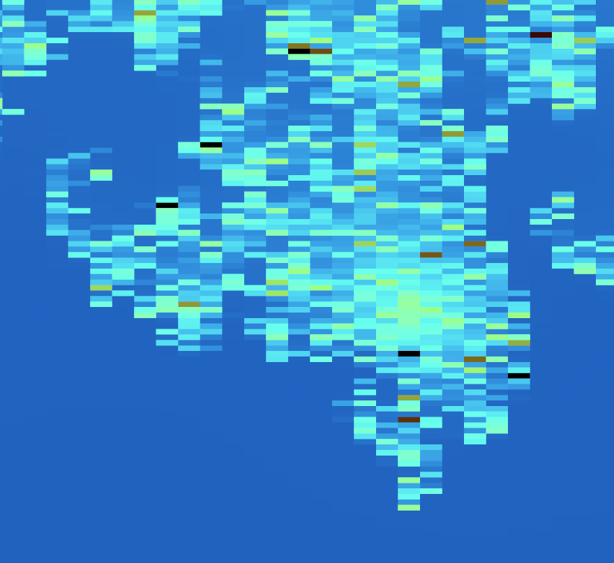
Fig. 3: The Mandelbrot fractal, when zooming in deeper than 32-bit floating-point precision allows
Antialiasing
Mapping each pixel to the complex coordinate that lies over the centre of the pixel is a decent approximation of the fractal at the available resolution, and gives quite visually appealing results, as seen above. However, like many other implementations in computer graphics, it suffers from our eternal enemy, aliasing effects, as well as noise. Because a pixel covers a non-zero portion of the complex plane, sampling the fractal only at the centre may not produce the colour that best represents that area, it is not surprising that we see jagged curves and what looks like random noise. Ideally, we would sample the fractal across every infinitessimal point on the pixel (an integral) and compute their average color. In the absence of infinite computing power, we can do the next-best thing: Compute a number of samples, more than 1 but few enough that the application remains navigable in real-time. One easy way to do this is to subdivide the pixel uniformly into 4, 9 or more subpixels, and sample those. The average colour of all subpixels becomes the final colour of the original pixel. The approach is obviously computationally expensive but easy to implement and yields much better visual results:
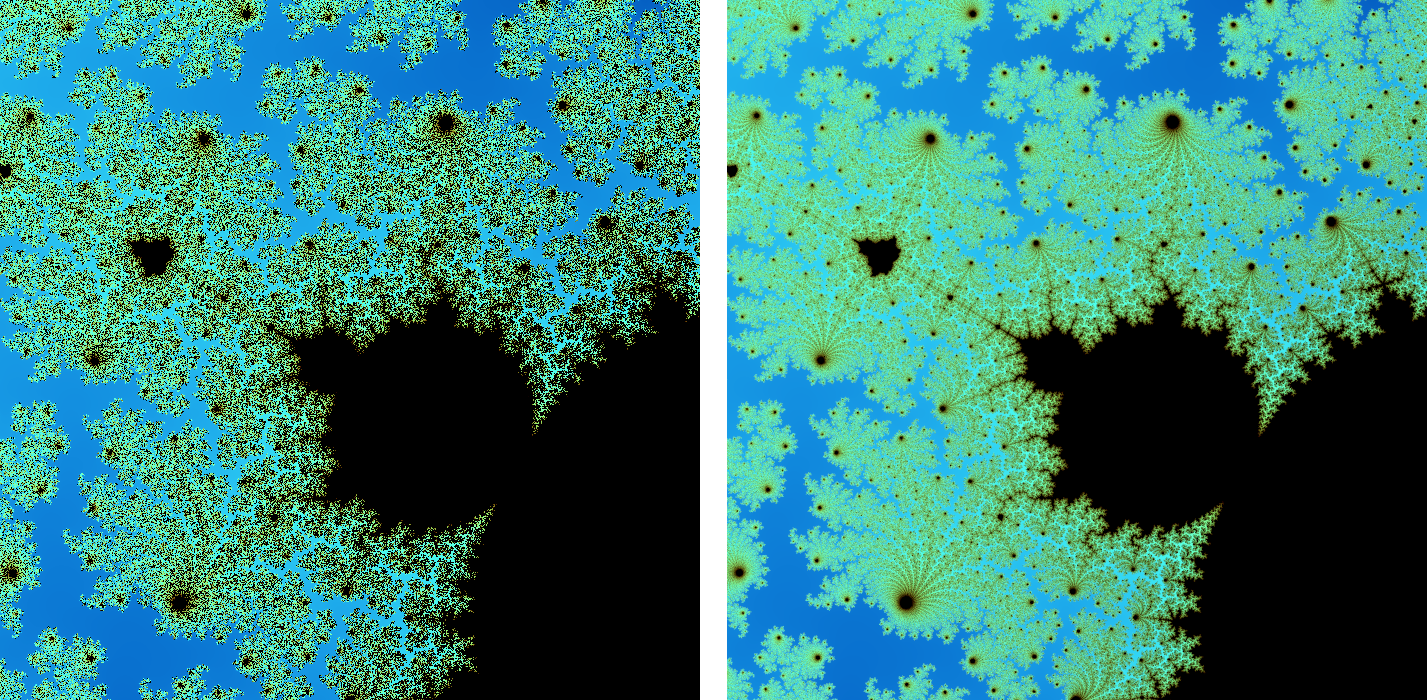
Fig. 4: A portion of the Mandelbort fractal with no antialiasing (left) and 5x5 supersampling (right)
The amount of supersampling is simply exposed as a parameter to balance, together with resolution and iteration count, with the desired visual quality and framerate. On powerful modern hardware, this demo can run in relative real-time with all settings on maximum, but on less powerful devices, such as mobile devices, the settings must be tuned down a little.
The main() function of the fragment shader was implemented as follows:
void main() {
    float aspect = viewSize.x / viewSize.y;
    vec3 color = vec3(0.0);

    for (int i=0; i<AA; ++i) {
        for (int j=0; j<AA; ++j) {

            vec2 virtualCoord = (float(AA) * vec2(gl_FragCoord) + vec2(i, j)) / (float(AA) * viewSize);
            virtualCoord -= 0.5;
            virtualCoord *= 2.0;
            vec2 c = zoomTarget + zoomRadius * virtualCoord * vec2(aspect, 1.0);
            color += getFractalColor(mandelbrot(c));

        }
    }

    color /= float(AA * AA);
    gl_FragColor = vec4(color, 1.0);
}
Julia Fractal
With the Mandelbrot fractal renderer implemented, it is very easy to add support to certain other fractals with similar implementations. One such fractal is the famous Julia set. We can render some hand-picked special cases of the Julia fractal using essentially the same algorithm as for the Mandelbrot set. To render the Mandelbrot fractal, our spatial variable was
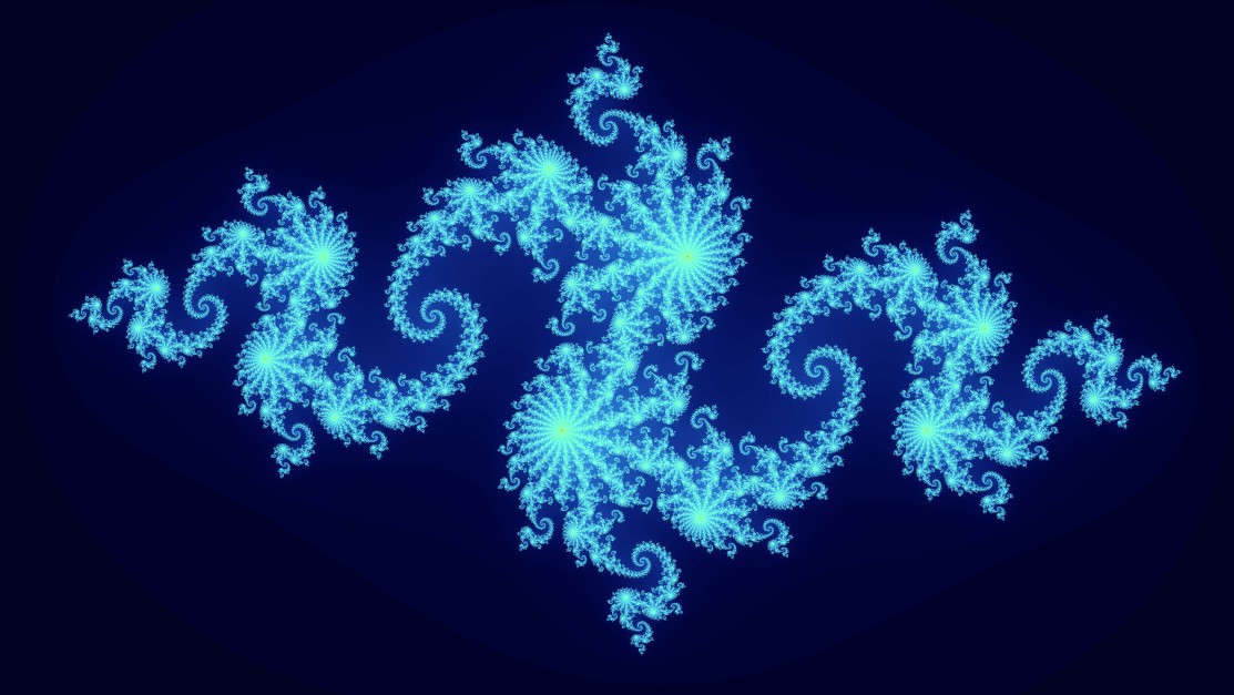
Fig. 5: Julia fractal for
The Julia fractal can look wildly different for various constants
And that concludes this coding adventure. The result is a satisfying little fractal navigator that lets the user explore this beautiful hidden corner of mathematics.