Particle System
This demo features an interactive particle system, where particles flow around according to some physics-inspired laws and interact with mouse/touch movements in real-time. The goal here is not to simulate anything out of reality, but rather something that is satisfying to play around with. A bit of digital art.
Simulation
We can simulate a simple gravitational field around the cursor by digging up Newton's law of universal gravitation:
If we imagine that all particles have some small "mass", and the cursor has a very large one, we can ignore any gravitational effect that particles would have on each other — conveniently turning the problem from a computationally hard one to a trivial one. All particles can now be processed independently in parallel, and they only need to be aware of their own state and the cursor position. By inserting the equation above into another classical Newtonian equation:
where
Having obtained an expression for the acceleration of each particle at any point in time, what is left is simply to keep track of the position and velocity for each particle. We can express the situation with a simple differential equation with respect to time
But since we are programming for the discrete world, we can spare ourselves the more rigorous calculus and solve it numerically, for each frame as follows:
where
which is already clear enough to serve as our pseudocode.
WebGL implementation
The system supports particle counts in the order of millions — on powerful hardware hundreds of millions. To achieve this, not only the rendering but also the computation is done on the GPU, in WebGL. Rendering points in WebGL is straight-forward using the pipeline as intended - the vertex shader calculates the position and the fragment shader draws the point with a desired colour. However, the particle simulation step requires some additional thought. For each frame, we want each particle to remember its previous position (and maybe some additional parameters like velocity or acceleration), and update itself for the current frame. But in WebGL, this is not possible in a single render pass: The vertex shader does not have a way to keep track of such a state.
The solution is to have two separate render passes, one for computation and one for rendering. In our compute pass, we essentially need to trick WebGL that we are drawing something visually useful, where actually the output is just data that we never show. Instead of rendering it to the screen, we render it into a texture that we then give as input to our second pass.
The compute pass consists of a simple unit quad, rendered directly onto the render target. We make the render target have at least the same size as the number of particles in our system, so that each pixel corresponds to one particle. Then we clone the render target, so that we can swap between them on each frame: One is the input, the other is the output, and the next frame they swap places. This way, we can feed the previous frame's state into the shader of the current compute pass, which can read the previous state, make its changes and output the new state. The render pass will then use the new state as input to render the particles.
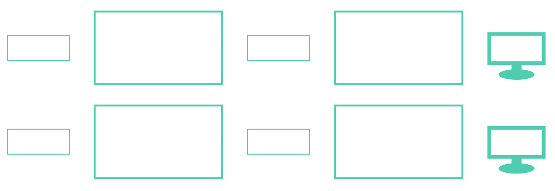
Fig. 1: A diagram over how two consecutive frames are rendered, using the data textures in between. Between each frame, the textures swap places.
We can choose the datatype of the data texture pixels, so we are not limited to single-byte precision per colour channel, but we are still limited by the number of channels. This demo uses the RGBA format with 32-bit floating point precision. In other words, there's not a lot of room on board: We must make the particle state fit into a 4-dimensional vector with f32-typed components. Luckily, that's all the room we need. Since the particles exist in two dimensions, we can encode its position and velocity into the output pixel as follows:
Since acceleration is recomputed for every frame and only depends on the particle and cursor positions, this state is all we need to implement the simulation described above. In actual GLSL shader code, our compute pass might look roughly like this:
int i = int(gl_FragCoord.x);
int j = int(gl_FragCoord.y);
vec4 state = texelFetch(prevState, ivec2(gl_FragCoord.xy), 0);
vec2 p = state.rg;
vec2 v = state.ba;

vec2 r = mousePos - p;
float dist = length(r);

vec2 a = alpha / (dist * dist * dist) * r;
v += delta * a;
p += delta * v;

gl_FragColor = vec4(p, v);
And apart from some boilerplate, as well as the damping and clamping mentioned earlier, that's how it looks.
The next step is to actually render the particles. The easiest way is to use WebGL point primitives. They each correspond to a single vertex with a vertex shader, which can set the position and screen-size of each point. The fragment shader is then run for each pixel inside that area. Normally, the position would be given as an attribute that the vertex shader then transforms in some deterministic manner, but in our case we will ignore the position attribute and instead read out the particle state for the current vertex from our newly updated data texture, as follows:
precision highp float;

uniform int texWidth;
uniform float pointSize;
uniform sampler2D currState;

flat out vec2 v;

void main() {
    ivec2 coord = ivec2(gl_VertexID % texWidth, gl_VertexID / texWidth);
    vec4 state = texelFetch(currState, coord, 0);

    gl_PointSize = pointSize;
    gl_Position = vec4(state.rg, 0.0, 1.0);
    v = state.ba;
}
And that's it! The particle system will now work, as long as the fragment shader outputs some visible colour. To make things more interesting (and prettier), we choose this colour based on the speed of the particle, so that faster particles will be rendered with a brighter colour. To achieve this, we output the velocity as a varying to the fragment shader. By making the particles slightly transparent, we get a nicer, smoke-like effect when the number of points is large enough for the resolution:
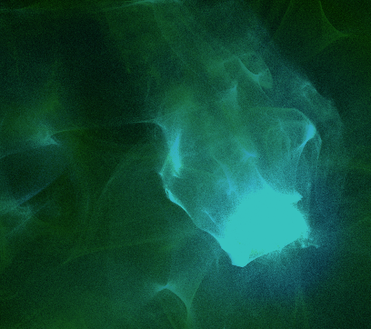
Fig. 2: Smoke-like effect when setting a high point density but a low opacity
As playing around with these parameters is meant to be part of the user experience, the demo exposes a few more as settings:
- A particle size, which makes particles larger than the single-pixel default, shaded as blurry spheres
- A 'viscosity' setting that changes how much dampling is applied. Low damping makes the system faster but less stable, higher damping makes it resemble a viscous fluid.
- A border bounce setting, which makes particles reflect away form the borders instead of continuing in and out of view
- A colour scheme, which changes the base colours of particles at different speeds